2DOF Systems
The 2DOF (Two Degree of Freedom) systems module in nphmu_vmd allows for the analysis of systems with two or more degrees of freedom. This section provides a guide on using the MDOF systems module, including quick examples and detailed tutorials.
Quick Examples
To get a feel for how the 2DOF systems module works, here are a few quick examples.
Example 1: Basic Usage
Import the basic sdof module and numpy and plotting capabilities
import numpy as np
import matplotlib.pyplot as plt
from np_vmd.tdof_MCK import TDOF_modal
Define a system 2DOF system with
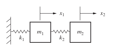
m1 = 9 and m2=1 kg
c1 = 2.4 and c=0.3 kg/s
k1 = 24 and k2=3 N/m
The equation of motion in matrix form is:
The connection between the elements determines:
Mmat: Inertial matrix
Cmat: Damping matrix
Kmat: Stiffness matrix
m1,m2  = 9,1
k1=24
k2=3
c1 = 2.4
c2 = 0.3
# definition of system matrices.
Mmat = np.array([[m1,0],[0,m2]])
Kmat = np.array([[k1+k2,-k2],[-k2,k2]])
Cmat =  np.array([[c1+c2,-c2],[-c2,c2]])
# system definition
tmck = TDOF_modal(Mmat, K=Kmat, C=Cmat)
Next is the initial excitation and the initial values. In this example wi are setting:
x1 = 1 and x2 = 0 (initial displacement only for mass 1)
x’1=0 and x’2 = 0 (initial velocity is 0)
tmck.set_iv(x0s = np.array([[1, 0]]).T, dx0s = np.array([[0,0]]).T)
It possible to obtain the intermediate uncoupled matrices (optional) and other relevant values
print(f"K-tilde:\n {tmck.Ktilde}")
print(f"zs     : {tmck.zs}")
tmck.update_damping( np.array([0.1, 0.05]))
print(f"zs     : {tmck.zs}")
print(f"wns     : {tmck.wns}")
Example 2: calculate the Free Response
Continuing from above:
define a time vector t
obtain the free response (displacement)
plot the free response
plot the velocity respone:
ts = np.linspace(0, 50, 1000) # time vector
xs = tmck.calc_x_hom_response(ts) # positions

fig, axs = plt.subplots(2,1, sharex=True, sharey=True)
axs[0].plot(ts, xs[0,:], label = 'x_1')
axs[1].plot(ts, xs[1,:], label = 'x_2')
axs[0].legend()
axs[1].legend()
plt.xlabel('time [s]')
axs[0].set_ylabel('$x_1$')
axs[1].set_ylabel('$x_2$')
plt.show()
Detailed Tutorials (WIP)
Here we walk through detailed examples of common analyses you can perform with the SDOF module.
Example 1: Detailed Analysis of an 2DOF System
# Detailed tutorial content